Santa Barbara Scientific SM-2 Seeing Monitor

The SBS SM-2 Seeing Monitor utilizes a high QE, low noise CMOS sensor and a high quality 100mm f/3.5 lens as well as custom seeing monitor software written by Dr. Alan Holmes.  The Seeing Monitor constantly monitors the seeing for any 12 hour period and displays the measurement on the computer monitor, logging the data to a text file for later analysis.  The camera is mounted in a weather resistant aluminum box with an optical quality window for protection from the elements.  With the cover removed, the camera may be focused and the pointing is independently adjustable.  Computer interface is USB2.  There is room for a powered USB extender to be installed in the aluminum housing either underneath or behind the camera.

SM2 DETAILS

The SM-2 Seeing Monitor is mechanically indentical to the former SM-1 model.  Internally, however, the SM-2 uses a new sensor and new lens.  The new sensor is the 1.2 Megapixel MT9M034 CMOS with exceptionally high (74%) QE and exceptionally low (~5e-) read noise.  The sensor's on-chip FPN (Fixed Pattern Noise) calibration function solves one of the major problems of CMOS technology, resulting in images that are clear and uniform, even under high gain.   The new lens is a high quality Japanese made 100mm f/3.5 c-mount lens that is ideal for this application. 

The SM-2 seeing monitor is particularly useful for those with a permanent installation, but also useful for those who must set up each night to take astro images.  By reporting and charting the seeing from night to night and from hour to hour, the user can determine the optimum time to attempt high resolution images and the times when perhaps equipment better suited to wide field, lower resolution imaging would be advisable.  The Seeing Monitor integrates necessary hardware in a weatherproof box and includes custom software.  The seeing is displayed in units of the zenith Full Width Half Maximum (FWHM) in arcseconds expected for a long exposure star image.

Theory of operation

Most professional observatories use the Differential Image Motion Monitor (DIMM) technique to measure seeing. This technique is implemented in hardware by using a two hole mask over an 8 to 11 inch Schmidt-Cassegrain telescope aperture, and measuring the root mean square (rms) fluctuation of the spacing of the two spots seen when a bright star is imaged a little bit out of focus with a fast camera. The reason two spots are measured is that the aggregate motion of the two spots due to poor tracking or wind vibration can therefore be rejected. However, the resulting system is complicated to automate, and invariably requires an automated enclosure to house the telescope as well, running the total cost up to many thousands of dollars.  One problem with this approach is that it completely ignores tube currents in the SCT, which are not small, nor correlated across the aperture. The approach used with the SBS Seeing Monitor is to use a fixed single aperture system staring at Polaris, mounted on a heavy solid pier. This way the wind motion and tracking error is gone. Polaris does move across the space of a measurement, so the linear drift of the centroid of Polaris’s position is determined and corrected. We call this the SIMM technique.  

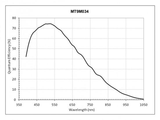
Figure Two: Two Summed Exposures of Polaris Field

An accurate seeing measurement requires exposures of 0.01 seconds or faster to freeze the seeing, and avoid errors due to the star motion being average over a long exposure. In the case of the SM-2, the software collects 256 frames of date, each with an exposure of 0.01 second.  The rms image motion is then determined. 256 frames requires about a minute of time to collect and process.  A high quality lens (Fig. One, above) with a focal length of 100 mm will achieve sub-pixel accuracy with the centroid calculation, and the motion of Polaris over a night can be contained on the CMOS sensor with a 100 mm focal length.  Over the course of a night Polaris may move in a 180 degree arc, so its motion must be considered for any long term monitoring plan.

At the latitude of Santa Barbara, CA (35 degrees) the noise floor of an SM-2 with a 100 mm lens is about 0.6 arcseconds FWHM.  This is measured indoors at night by viewing an LED of brightness comparable to Polaris, being driven slowly in a horizontal direction. Understand that this low value will be added in an rms sense to the actual seeing at low levels. So, if an SM-2 with a 100 mm lens measures 1.0 arcsecond seeing, one needs to subtract the 0.6 second measured bias from this (in an rms sense) to give the actual seeing, 0.8 arcseconds.  Converting the measured seeing at the elevation of Polaris into a zenith value is done using a well-accepted formula, where the seeing at the zenith is equal to the seeing measured for Polaris divided by the airmass to the 0.6 power. Airmass is equal to 1 divided by the cosine of the quantity 90 degrees minus the latitude.

Figure Three: Setup Menu

Seeing Monitor Menu: here you can choose to immediately start logging the seeing. If you want to start at a specific time select Timed Based and the program will execute for the period commanded. When logging begins, a graph displaying the zenith FWHM (full width half maximum of the star image) will pop up, with a start time which is the previous hour’s number, and that shows 12 hours of data. The length of this graph is fixed at 12 hours.  The graph, and a text file logging the seeing data will be written to the C:\SeeingMonitor directory every 5 minutes. The seeing graph name never changes, so you can have an external program monitor this folder and put the file up on a web site, if you wish. The logged data file name is the same every time if you start immediate logging, and will overwrite the last night’s file, so change the previous night’s text file name manually if you wish to save it. When operating in a multi-night mode using a timed start and finish the file name is customized with the date, so the previous night’s data will not be overwritten. The seeing graph is always overwritten.

Figure Four: Main Screen

Figure Five: Seeing Graph

On the graph shown in figure five, above, the white data points record the seeing number in arc seconds.  The blue data points represent the brightness of polaris at the time of each measurement.  You can see from the graph that on this night the seeing began to deteriorate around 3:00AM and got rapidly worse over the next 45 minutes until it was useless to image.  The brightness of Polaris also began to deteriorate at the same time, which together indicates encroaching clouds or fog.  Even when sampling at 100 times a second, when the seeing is REALLY bad the seeing monitor is probably underestimating how bad it is since the image is just a boiling blob. Even though the seeing monitor underestimates these terrible nights, it provides a clear indication that you would be better off doing something other than astro-imaging that night.  The usefulness of the seeing monitor is readily displayed in the next Figure, below.  This is an animation of 13 graphs taken over a two week period.  As you can see, the seeing, and the patterns of good vs. poor seeing per night, vary a great deal making it almost impossible to rely on history or experience to predict when the night will be worthy of hour long exposure efforts, or not.